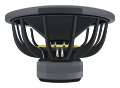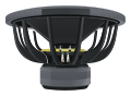
Piston radiation impedance.
Evaluate the one-sided acoustic radiation impedance of a rigid circular piston in an infinite baffle, including a numerically stable low-frequency limit.

Piston geometry
Operating point
Air & conventions
One-sided acoustic radiation impedance
LOG FREQUENCYDo not add this mass to manufacturer Mms without reconciling its existing air-load convention.
Read this result with its assumptions.
Ideal rigid circular piston in an infinite baffle, one radiating side. Acoustic impedance is pressure divided by volume velocity.
The low-frequency mass approximation is appropriate only when ka is much smaller than one.
Units & assumptionsYour calculations run in this browser. No account needed.
The math, in plain sight.
The air in front of the cone is part of the load.
One side of a baffled rigid piston
For piston radius a, area S, and wavenumber k, the acoustic impedance is pressure divided by volume velocity. J1 is the Bessel function and H1 is the Struve function.
The stable low-frequency approximation
The implementation uses the leading-order form for ka below 0.001 to avoid subtracting nearly equal values. Otherwise it evaluates stable integral representations with composite Simpson quadrature. The numerical operating-point limit is ka = 100.
Mathematical series and model boundary
Manufacturer moving mass commonly includes an air-load convention. Do not simply add the calculated radiation mass to published Mms. Cone breakup, finite baffles, enclosure edges, and noncircular diaphragms lie outside this model.